## Decoding Patient Health Trajectories with EHRFormer: A Deep Dive into Methodology
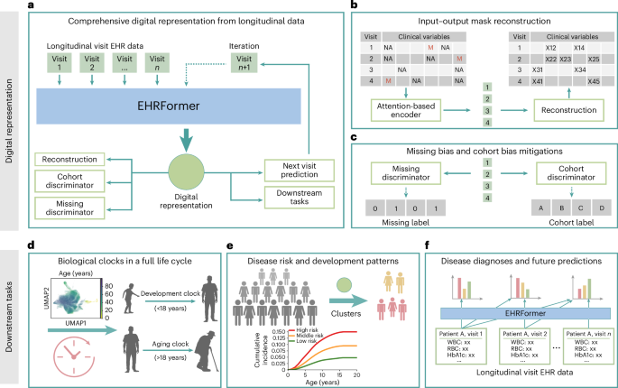
Electronic Health Records (EHRs) hold a wealth of information,but unlocking their predictive power requires elegant analytical approaches. Our recent work leverages a novel deep learning model, EHRFormer, to extract meaningful insights from these complex datasets, ultimately aiming to improve disease prediction and personalized healthcare. This article provides a detailed overview of the methodologies employed in our research, offering transparency and reproducibility for the wider scientific community.### Data Preprocessing and feature Engineering
The foundation of any successful machine learning project lies in robust data planning. We began by meticulously processing a large-scale EHR dataset, focusing on laboratory measurements and vital signs – key indicators of a patient’s health status. These features were then standardized to ensure consistent scaling and prevent any single variable from disproportionately influencing the model.
A crucial aspect of our approach involved calculating a “raw age difference.” This metric, represented as Δi = Ab,i – f(Ac,i), quantifies the deviation of a patient’s developmental trajectory from that of their healthy peers, considering chronological age (CA). Here, Ab,i represents a specific biomarker value for patient *i*, and f(Ac,i) is a function predicting the expected biomarker value based on their CA.This allows us to identify individuals who are developing at a rate significantly different from the norm.
To further refine this measure, we standardized these raw age differences by dividing them by the standard deviation (σ) within our model, resulting in a z-score (zi = Δi / σ). This standardization allows for a more direct comparison of deviations across different biomarkers and patients.### Unveiling Hidden Patterns: Latent Space Visualization and Clustering
EHRFormer generates high-dimensional “latent vectors” that encapsulate a patient’s overall health profile. To make these complex representations interpretable, we employed several dimensionality reduction and visualization techniques.
First, we used Principal Component Analysis (PCA) with 50 components to reduce the dimensionality of the latent vectors while preserving the most vital information. This simplified representation was then further processed using a neighbor graph approach – identifying the 15 nearest neighbors for each data point based on Euclidean distance.
We then leveraged Uniform Manifold Approximation and projection (UMAP), a powerful non-linear dimensionality reduction technique (parameters: min_dist=0.3,spread=1.0, 2 components, spectral initialization), to visualize these relationships in a two-dimensional space. This visualization revealed distinct clusters of patients.
To identify these clusters, we applied the Leiden community detection algorithm. Interestingly, the resulting clusters largely corresponded to pediatric and adult populations, suggesting that EHRFormer was effectively capturing age-related differences in health trajectories.
### Disease Risk Assessment within Patient Subgroups
Once we identified these patient clusters, we investigated disease prevalence and incidence within each group. *Prevalence* was defined as the proportion of individuals with a pre-existing condition at their first hospital encounter, providing a snapshot of baseline disease burden. *Incidence*, on the othre hand, measured the proportion of initially healthy individuals who developed the condition within a five-year follow-up period.
By visualizing these prevalence and incidence proportions within each cluster, we were able to identify patient subgroups with a disproportionately high risk of specific diseases. This allows for targeted interventions and preventative care strategies.
### Quantifying Disease Associations: Adjusted Hazard Ratios
To rigorously quantify the association between cluster membership and disease risk, we calculated adjusted log2 Hazard Ratios (HRs).Using Cox proportional hazards models, we compared the risk of disease in each cluster to the remainder of the study population.
Crucially, these models were adjusted for potential confounding factors, including patient demographics (age and sex), smoking history, alcohol consumption, and hospital affiliation. This ensures that the observed associations are more likely to reflect a true relationship between cluster membership and disease risk. To enhance interpretability, log2HR values were truncated at a maximum of 2, focusing on the most significant associations. HRs were calculated using the lifelines Python package (version 0.30.0).
### Model Evaluation and Statistical Rigor
Throughout our analysis, we adhered to rigorous statistical standards. Regression models for continuous value predictions were evaluated using Mean absolute Error (MAE), R-squared (R), and Pearson Correlation Coefficient (PCC). Binary classification models were assessed using Receiver operating Characteristic (ROC) curves, with the Area Under the Curve (AUC) reported along with 95% confidence intervals. AUCs were
Related reading